Cubic response functions: *CCCR

In the *CCCR section the input that is specific for coupled cluster cubic response properties is read in. This section includes:

• frequency-dependent fourth-order properties
  
  $$\gamma_{ABCD}(\omega_A;\omega_B,\omega_C,\omega_D) = - \lang... ... \quad \mbox{with~} \omega_A = -\omega_B -\omega_C -\omega_D$$
  
  
  where $A$, $B$, $C$ and $D$ can be any of the one-electron operators for which integrals are available in the **INTEGRALS input part.
• dispersion coefficients $D_{ABCD}(l,m,n)$ for $\gamma_{ABCD}(\omega_A;\omega_B,\omega_C,\omega_D)$ which for $n \ge 0$ are defined by the expansion
  
  $$\gamma_{ABCD}(\omega_A;\omega_B,\omega_C,\omega_D) = \sum_{... ...infty} \omega_B^l \, \omega_C^m \, \omega_D^n D_{ABCD}(l,m,n)$$
  
  

Coupled cluster cubic response functions and dispersion coefficients are implemented for the models CCS, CC2 and CCSD.

The response functions are evaluated for a number of operator quadruples (specified with the keywords .OPERAT, .DIPOLE, or .AVERAG) which are combined with triples of frequency arguments specified using the keywords .MIXFRE, .THGFRE, .ESHGFR, .DFWMFR, .DCKERR, or .STATIC. The different frequency keywords are compatible and might be arbitrarely combined or repeated. For dispersion coefficients use the keyword .DISPCF.

.AVERAG

READ (LUCMD,'(A)') AVERAGE
READ (LUCMD,'(A)') SYMMETRY

Evaluate special tensor averages of cubic response functions. Presently implemented are the isotropic averages of the second dipole hyperpolarizability $\gamma_{\vert\vert}$ and $\gamma_{\bot}$. Set AVERAGE to GAMMA_PAR to obtain $\gamma_{\vert\vert}$ and to GAMMA_ISO to obtain $\gamma_{\vert\vert}$ and $\gamma_{\bot}$. The SYMMETRY input defines the selection rules exploited to reduce the number of tensor elements that have to be evaluated. Available options are ATOM, SPHTOP (spherical top), LINEAR, and GENER (use point group symmetry from geometry input). Note that the .AVERAG option should be specified in the *CCCR section before any .OPERAT or .DIPOLE input.

.DCKERR

READ (LUCMD,*) MFREQ
READ (LUCMD,*) (DCRFR(IDX),IDX=NCRFREQ+1,NCRFREQ+MFREQ)

Input for dc-Kerr effect $\gamma_{ABCD}(-\omega;0,0,\omega)$: on the first line following .DCKERR the number of different frequencies are read, from the second line the input for $\omega_D = \omega$ is read. $\omega_B$ and $\omega_C$ to $0$ and $\omega_A$ to $-\omega$.

.DFWMFR

READ (LUCMD,*) MFREQ
READ (LUCMD,*) (BCRFR(IDX),IDX=NCRFREQ+1,NCRFREQ+MFREQ)

Input for degenerate four wave mixing $\gamma_{ABCD}(-\omega;\omega,\omega,-\omega)$: on the first line following .DFWMFR the number of different frequencies are read, from the second line the input for $\omega_B = \omega$ is read. $\omega_C$ is set to $\omega$, $\omega_D$ and $\omega_A$ to $-\omega$.

.DIPOLE

Evaluate all symmetry allowed elements of the second dipole hyperpolarizability (max. 81 components per frequency).

.DISPCF

READ (LUCMD,*) NCRDSPE

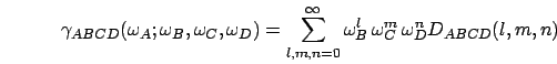
Calculate the dispersion coefficients $D_{ABCD}(l,m,n)$ up to $l+m+n =$ NCRDSPE. Note that dispersion coefficients presently are only available for real fourth-order properties.

.ESHGFR

READ (LUCMD,*) MFREQ
READ (LUCMD,*) (BCRFR(IDX),IDX=NCRFREQ+1,NCRFREQ+MFREQ)

Input for electric field induced second harmonic generation $\gamma_{ABCD}(-2\omega;\omega,\omega,0)$: on the first line following .ESHGFR the number of different frequencies are read, from the second line the input for $\omega_B = \omega$ is read. $\omega_C$ is set to $\omega$, $\omega_D$ to $0$ and $\omega_A$ to $-2\omega$.

.L2 BC

solve response equations for the second-order Lagrangian multipliers $\bar{t}^{BC}$ instead of the equations for the second-order amplitudes $t^{AD}$.

.L2 BCD

solve response equations for the second-order Lagrangian multipliers $\bar{t}^{BC}$, $\bar{t}^{BD}$, $\bar{t}^{CD}$ instead of the equations for the second-order amplitudes $t^{AD}$, $t^{AC}$, $t^{AB}$.

.MIXFRE

READ (LUCMD,*) MFREQ
READ (LUCMD,*) (BCRFR(IDX),IDX=NCRFREQ+1,NCRFREQ+MFREQ)
READ (LUCMD,*) (CCRFR(IDX),IDX=NCRFREQ+1,NCRFREQ+MFREQ)
READ (LUCMD,*) (DCRFR(IDX),IDX=NCRFREQ+1,NCRFREQ+MFREQ)

Input for general frequency mixing $\gamma_{ABCD}(\omega_A;\omega_B,\omega_C,\omega_D)$: on the first line following .MIXFRE the number of differenct frequencies is read and from the next three lines the frequency arguments $\omega_B$, $\omega_C$, and $\omega_D$ are read ($\omega_A$ is set to $-\omega_B-\omega_C-\omega_D$).

.NO2NP1

test option: switch off $2n+1$-rule for second-order Cauchy vector equations.

.OPERAT

READ (LUCMD,'(4A)') LABELA, LABELB, LABELC, LABELD
DO WHILE (LABELA(1:1).NE.'.' .AND. LABELA(1:1).NE.'*')
READ (LUCMD,'(4A)') LABELA, LABELB, LABELC, LABELD
END DO

Read quadruples of operator labels. For each of these operator quadruples the cubic response function will be evaluated at all frequency triples. Operator quadruples which do not correspond to symmetry allowed combination will be ignored during the calculation.

.PRINT

READ (LUCMD,*) IPRINT

Set print parameter for the cubic reponse section.

.STATIC

Add $\omega_A = \omega_B = \omega_C = \omega_D = 0$ to the frequency list.

.THGFRE

READ (LUCMD,*) MFREQ
READ (LUCMD,*) (BCRFR(IDX),IDX=NCRFREQ+1,NCRFREQ+MFREQ)

Input for third harmonic generation $\gamma_{ABCD}(-3\omega;\omega,\omega,\omega)$: on the first line following .THGFRE the number of different frequencies is read, from the second line the input for $\omega_B = \omega$ is read. $\omega_C$ and $\omega_D$ are set to $\omega$ and $\omega_A$ to $-3\omega$.

.USECHI

test option: use second-order $\chi$-vectors as intermediates

.USEXKS

test option: use third-order $\xi$-vectors as intermediates