Quadratic response functions: *CCQR

In the *CCQR section you specify the input for coupled cluster quadratic response calculations. This section includes:

• frequency-dependent third-order properties
  
  $$\beta_{ABC}(\omega_A;\omega_B,\omega_C) = - \langle\langle A... ...mega_C} \qquad \mbox{with~} \omega_A = -\omega_B - \omega_C$$
  
  
  where $A$, $B$ and $C$ can be any of the one-electron operators for which integrals are available in the **INTEGRALS input part.
• dispersion coefficients $D_{ABC}(n,m)$ for third-order properties, which for $n \ge 0$ are defined by the expansion
  
  $$\beta_{ABC}(-\omega_B-\omega_C;\omega_B,\omega_C) = \sum_{n,m=0}^{\infty} \omega_{B}^n \, \omega_{C}^m \, D_{ABC}(n,m)$$
  
  

The coupled cluster quadratic response function is at present implemented for the coupled cluster models CCS, CC2 and CCSD.

The response functions are evaluated for a number of operator triples (given using the .OPERAT, .DIPOLE, or .AVERAG keywords) which are combined with pairs of frequency arguments specified using the keywords .MIXFRE, .SHGFRE, .ORFREQ, .EOPEFR or .STATIC. The different frequency keywords are compatible and might be arbitrarily combined or repeated. For dispersion coefficients use the keyword .DISPCF.

.AVERAG

READ (LUCMD,'(A)') LINE

Evaluate special tensor averages of quadratic response properties. Presently implemented are only the vector averages of the first dipole hyperpolarizability $\beta_{\vert\vert}$, $\beta_{\bot}$ and $\beta_K$. All three of these averages are obtained if HYPERPOL is specified on the input line that follows .AVERAG. The .AVERAG keyword should be used before any .OPERAT or .DIPOLE input in the *CCQR section.

.DIPOLE

Evaluate all symmetry allowed elements of the first dipole hyperpolarizability (max. 27 components).

.DISPCF

READ (LUCMD,*) NQRDSPE

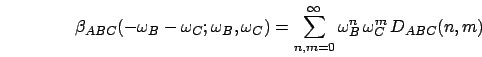
Calculate the dispersion coefficients $D_{ABC}(n,m)$ up to order $n+m =$NQRDSPE.

.EOPEFR

READ (LUCMD,*) MFREQ
READ (LUCMD,*) (BQRFR(IDX),IDX=NQRFREQ+1,NQRFREQ+MFREQ)

Input for the electro optical Pockels effect $\beta_{ABC}(-\omega;\omega,0)$: on the first line following .EOPEFR the number of different frequencies is read, from the second line the input for $\omega_B = \omega$ is read. $\omega_C$ is set to $0$ and $\omega_A$ to $\omega_A = -\omega$.

.MIXFRE

READ (LUCMD,*) MFREQ
READ (LUCMD,*) (BQRFR(IDX),IDX=NQRFREQ+1,NQRFREQ+MFREQ)
READ (LUCMD,*) (CQRFR(IDX),IDX=NQRFREQ+1,NQRFREQ+MFREQ)

Input for general frequency mixing $\beta_{ABC}(-\omega_B-\omega_C;\omega_B,\omega_C)$: on the first line following .MIXFRE the number of different frequencies (for this keyword) is read, from the second and third line the frequency arguments $\omega_B$ and $\omega_C$ are read ($\omega_A$ is set to $-\omega_B-\omega_C$).

.NOBMAT

Test option: Do not use B matrix transformations but pseudo F matrix transformations (with the zeroth-order Lagrange multipliers exchanged by first-order responses) to compute the terms $\bar{t}^A {\bf B} t^{B} t^{C}$. This is usually less efficient.

.OPERAT

READ (LUCMD'(3A)') LABELA, LABELB, LABELC
DO WHILE (LABELA(1:1).NE.'.' .AND. LABELA(1:1).NE.'*')
READ (LUCMD'(3A)') LABELA, LABELB, LABELC
END DO

Read triples of operator labels. For each of these operator triples the quadratic response function will be evaluated at all frequency pairs. Operator triples which do not correspond to symmetry allowed combination will be ignored during the calculation.

.ORFREQ

READ (LUCMD,*) MFREQ
READ (LUCMD,*) (BQRFR(IDX),IDX=NQRFREQ+1,NQRFREQ+MFREQ)

Input for optical rectification $\beta_{ABC}(0;\omega,-\omega)$: on the first line following .ORFREQ the number of different frequencies is read, from the second line the input for $\omega_B = \omega$ is read. $\omega_C$ is set to $\omega_C = -\omega$ and $\omega_A$ to $0$.

.PRINT

READ (LUCMD,*) IPRINT

Set print parameter for the quadratic response section.

.SHGFRE

READ (LUCMD,*) MFREQ
READ (LUCMD,*) (BQRFR(IDX),IDX=NQRFREQ+1,NQRFREQ+MFREQ)

Input for second harmonic generation $\beta_{ABC}(-2\omega;\omega,\omega)$: on the first line following .SHGFRE the number of different frequencies is read, from the second line the input for $\omega_B = \omega$ is read. $\omega_C$ is set to $\omega$ and $\omega_A$ to $-2\omega$.

.STATIC

Add $\omega_A = \omega_B = \omega_C = 0$ to the frequency list.

.USE R2

Test option: use second-order response vectors instead of first-order Lagrange multiplier responses.

.XYDEGE

Assume X and Y directions as degenerate in the calculation of the hyperpolarizability averages (this will prevent the program to use the components $\beta_{zyy}$, $\beta_{yzy}$ $\beta_{yyz}$ for the computation of the vector averages).